How to cross-validate PCA, clustering, and matrix decomposition models

This post was updated on 09/17/2019

Cross-validation in Linear Regression

Cross-validation is a fundamental paradigm in modern data analysis. However, it is largely applied to supervised settings, such as regression and classification. Here, the procedure is simple: fit your model on, say, 90% of the data (the training set), and evaluate its performance on the remaining 10% (the test set). However, this idea does not easily extend to other unsupervised methods, such as dimensionality reduction methods or clustering.

It is easiest to see why visually. Take a simple linear regression problem:

Here, \(\mathbf{A}\) is a \(m \times n\) matrix, $\mathbf{x}$ is vector with $n$ elements, \(\mathbf{b}\) is a vector containing $m$ elements. This model has $n$ parameters (the elements of \(\mathbf{b}\)) and \(m\) datapoints. Rows of $\mathbf{A}$ correspond to independent/predictor variables, and elements of \(\mathbf{b}\) correspond to dependent variables.

The basic idea behind cross-validation (and related techniques, like bootstrapping) is to leave out datapoints and quantify the effect on the model. We can leave out rows of $\mathbf{A}$ and corresponding elements of $\mathbf{b}$. Critically, this leaves the length of $\mathbf{x}$ unchanged — there are still $n$ variables to predict, but the number of datapoints $m$ is smaller.

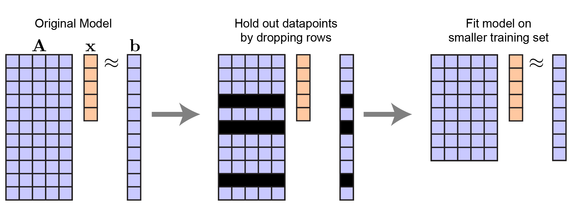Procedure to hold out data for linear regression. Note that $\mathbf{x}$ does not change in length.

To be explicit: let $\mathbf{A}_\text{tr}$ and $\mathbf{b}_\text{tr}$ respectively denote the training set of independent and dependent variables. Then fitting our model amounts to:

The beauty is that this reduces to the same optimization problem we started with (see equation 1). Furthermore, we know how to solve this particular problem very efficiently (see least-squares). After fitting the model, we can evaluate its performance on the held-out datapoints (i.e. the test set), which we denote $\mathbf{A}_\text{te}$ and $\mathbf{b}_\text{te}$. In the end we obtain an estimate of the generalization error of our model as $\lVert \mathbf{A}_\text{te} \hat{\mathbf{x}} - \mathbf{b}_\text{te} \lVert^2$.

This procedure is easily adapted to nonlinear regression models, of course.

Cross-validation in PCA

So what’s the problem with cross-validating PCA? I like to think of PCA as the following optimization problem:

This is much like linear regression, except we are optimizing over both $\mathbf{A}$ and $\mathbf{X}$ (which have been renamed to $\mathbf{U}$ and $\mathbf{V}^T$ to avoid confusion between the two models). Here, $\mathbf{Y}$ is a $m \times n$ matrix of data. In large-scale studies both $m$ and $n$ can be very high-dimensional and we may seek a simple low-dimensional linear model. This model is captured by $\mathbf{U}$ which is a tall-skinny matrix and $\mathbf{V}^T$ which is a short-fat matrix. Concretely, lets define $\mathbf{U}$ to me an $m \times r$ matrix and define $\mathbf{V}^T$ to be a $r \times n$ matrix, and choose $r$ to be less than $m$ and $n$. Then our model estimate $\hat{\mathbf{Y}} = \mathbf{U} \mathbf{V}^T$ is a rank-$r$ matrix

Some of you are probably grumpy that the above problem is not “really PCA” because PCA places an additional orthogonality constraint on the columns of $\mathbf{U}$ and $\mathbf{V}$. For a more careful discussion about the connection between PCA and equation 2 see my other post on PCA, this talk/tutorial I gave, and Madeleine Udell’s thesis work. Those resources also explain how nonnegative matrix factorization, clustering, and many other unsupervised models are also closely related to equation 2. Thus, our discussion of cross-validation will quickly generalize to these other very interesting models.

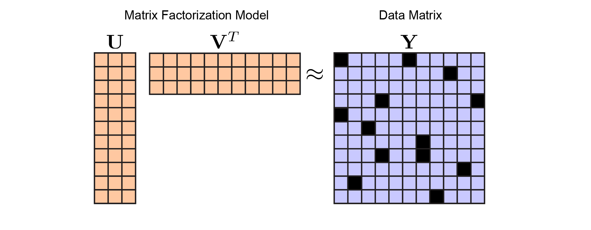
Once you are on board with the matrix factorization framework, you’ll see why cross-validation is tricky. Ultimately, our problem now looks like this:

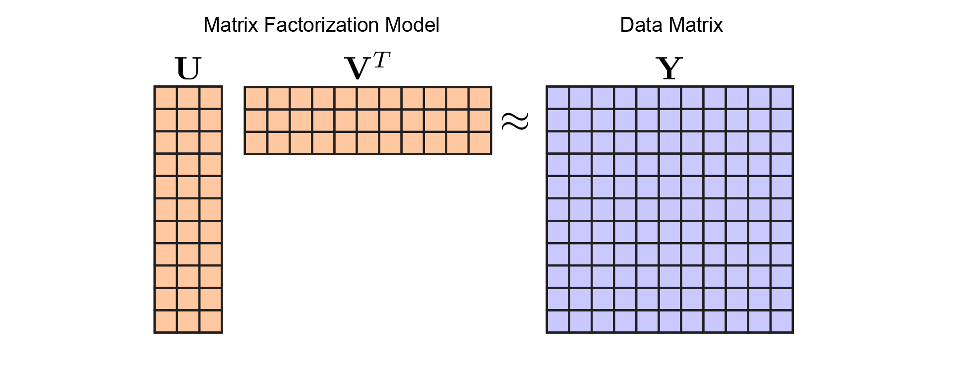Matrix Factorization Model. In keeping with figure 1, I've colored the model parameters (here, $\mathbf{U}$ and $\mathbf{V}$) in orange, while the data (here, $\mathbf{Y}$) is in blue. We optimize over $\mathbf{U}$ and $\mathbf{V}$ to minimize reconstruction error with respect to $\mathbf{Y}$

Ok, so how exactly should we hold out data in this setting? You might think we could leave out rows of $\mathbf{Y}$, however this would mean that you would have to leave out the corresponding row of $\mathbf{U}$. Thus, you couldn’t fit all of your model parameters! Likewise, leaving out a column of $\mathbf{A}$ would mean that you’d have to leave out a column of $\mathbf{V}^T$.

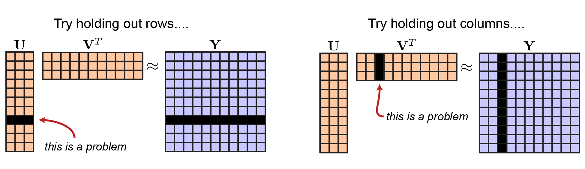Not so great ideas for cross-validating matrix factorization.

Maybe you only care about evaluating held-out/test error on our estimate of $\mathbf{V}$. That is, you don’t care about cross-validating $\mathbf{U}$ — you only care about cross-validating $\mathbf{V}$. Thus, you might suggest a two-step procedure in which we leave out rows of $\mathbf{Y}$ and fit $\mathbf{V}$ along with a subset of the rows of $\mathbf{U}$ on this training set. Then, to evaluate the performance of $\mathbf{V}$, we bend the rules of cross-validation ever so slightly and use the test set (held out rows) to fill out our estimate of $\mathbf{U}$.

Even this is not a good idea! It violates a core tenet of cross-validation that you don’t get to touch the the held out data. Your estimate of $\mathbf{V}$ could be horribly overfit, but by fitting $\mathbf{U}$ to on the test data, you could set these rows to zero and essentially blunt the effects of overfitting. Note that we have to fit this held out row of $\mathbf{U}$ in order to evaluate model performance along the corresponding row in the data matrix $\mathbf{Y}$ (which is the whole point of cross-validation).

Problems with holding out a whole column (or row) of the data matrix are discussed in more detail by Bro et al. (2008) and Owen & Perry (2009). Just in case you don’t believe me.

Why cross-validate PCA (and related methods)?

Before jumping into a solution, let’s remind ourselves why cross-validation is great and why applying it to PCA is a swell idea. In the case of regression and other supervised learning techniques, the goal of cross-validation is to monitor overfitting and calibrate hyperparameters. If we have a large number of regression parameters (i.e., $\mathbf{x}$ in equation 1 is a very long vector) then we’d commonly add regularization to the model. To take a very simple example, consider LASSO regression:

which will tend to produce an parameter estimate, $\hat{\mathbf{x}}$, that is sparse (containing many zeros). The scalar hyperparameter $\lambda > 0$ tunes how sparse our parameter estimate will be. If $\lambda$ is too large, then $\hat{\mathbf{x}}$ will very sparse and do a poor job of predicting $\mathbf{y}$. If $\lambda$ is too small, then $\hat{\mathbf{x}}$ will be not sparse at all, and our model could be overfit.

We can use cross-validation to estimate a good value for $\lambda$, by finding the value which minimizes the error of our model on the held-out test data. This procedure for model selection is machine learning 101 (see Chap. 7 in ESL). The basic picture looks like this:

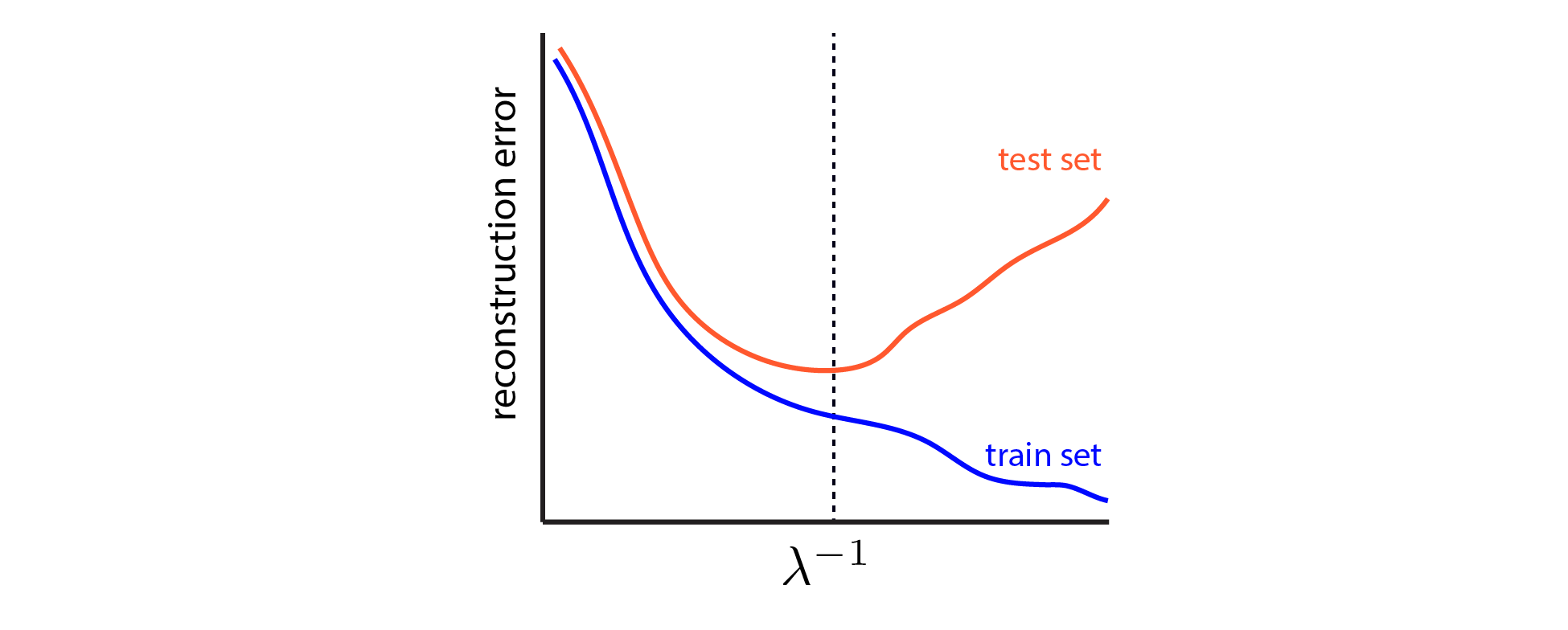Cross-validation schematic for LASSO dashed vertical line denotes the best value for $\lambda$, which achieves lowest error on the held-out test set.

For simplicity, I am glossing over the possibility of using a validation set as well as a test set. In short, if we pick $\lambda$ based on the minimum of the red curve above, then the test error will underestimate the genearlization error of the model. Here we won’t concern ourselves with estimating the generalization error directly — we just want to pick a good model. But it should be kept in mind that further splitting the data into training, validation, and test sets is the appropriate way to achieve unbiased estimates of out-of-sample performance.

In short, we can use cross-validation to tune model hyperparameters (e.g. $\lambda$ in LASSO). PCA also has an important hyperparameter — the number of components in the model. People have published a lot of papers on this (e.g. here, here, & here). Similarly, many clustering models require the user to choose the number of clusters prior to fitting the model. Choosing the number of clusters has also received a lot of attention. Viewed from the perspective of matrix factorization, these are the exact same problem – i.e. how to choose $r$, the width of $\mathbf{U}$ and the height of $\mathbf{V}^T$.

A cross-validation procedure for matrix decomposition

Without further ado, here are some plots that demonstrate how cross-validation can help you choose the number of components in PCA, NMF, and K-means clustering. In each example, I generated data from a ground truth model with $r=4$ and then added noise. That is, for PCA, the correct number of PCs was 4. For k-means clustering, the correct number of clusters was 4. From the test error, you can see that all models begin to overfit when $r>4$. From the training data alone, the cutoff is maybe not so clear.

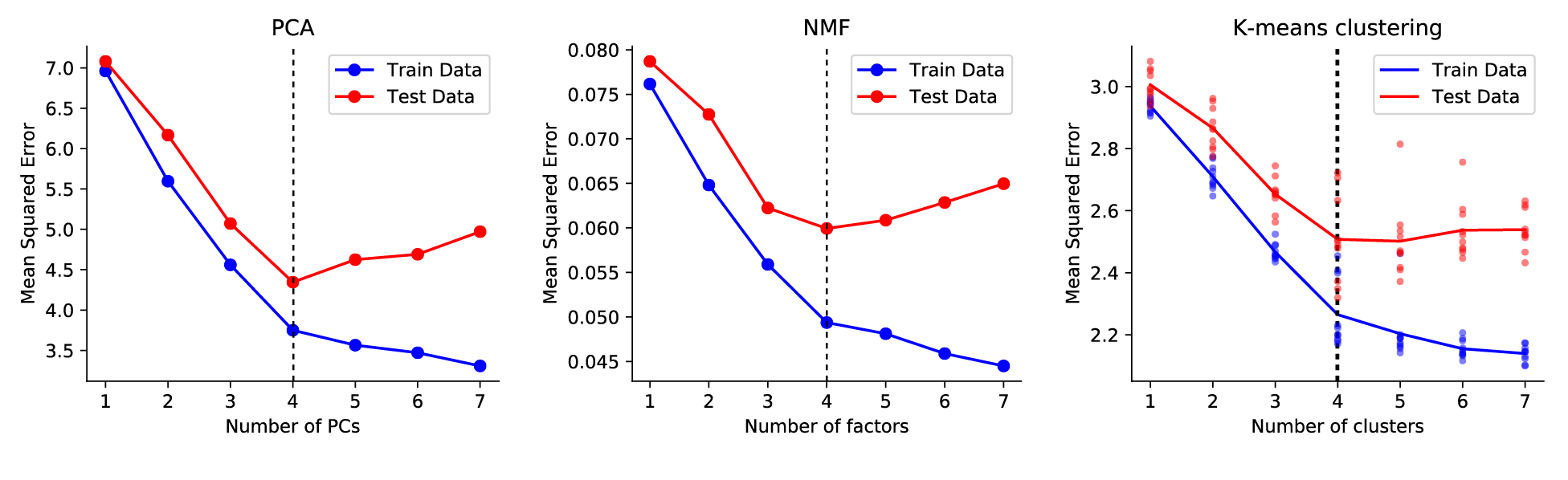Cross-validation plots for some matrix decomposition models. Note that the k-means implementation is a bit noisy so I averaged across multiple optimization runs. The code to generate these plots is posted here.

To make these plots I used a “speckled” holdout pattern (Wold, 1978). For simplicity and demonstration, I left out a small number of elements of $\mathbf{Y}$ at random:

A good solution is to hold out data at random. Importantly, we can still fit all parameters in $\mathbf{U}$ and $\mathbf{V}$ as long as no column or row of $\mathbf{Y}$ is fully removed. Intuitively, we should keep at least $r$ observations in each row or column.

Formally, we define a binary matrix $\mathbf{M}$, which acts as a mask over our data. That is every element in $\mathbf{M}$ is either $\mathbf{M}_{ij} = 0$, indicating a left out datapoint, or $\mathbf{M}_{ij}=1$, indicating a datapoint in the training set. We are left with the following optimization problem:

Where $ \circ $ denotes the Hadamard product. After solving the above optimization problem, we can then evaluate the error of our model on the held-out datapoints as: $\left \lVert (1-\mathbf{M}) \circ \left ( \mathbf{U} \mathbf{V}^T - \mathbf{Y} \right ) \right \lVert_F^2$.

We need not choose $\mathbf{M}$ to be random! We can select whatever holdout pattern we like, and indeed to ensure that all columns and rows are left out at equal rates we can leave out pseudo-diagonals of the matrix. In the interest of brevity and simplicity we will sweep these choices under the rug, but see Fig.1 in Wold (1978) for more discussion.

So how do we solve this optimization problem? As I mentioned before, equation 3 amounts to the well-studied low-rank matrix completion problem. However many papers that I’ve looked at do not provide algorithms for solving the problem in the particular form that we care about. In particular, they tend to optimize over a single matrix, call it $\hat{\mathbf{Y}}$, rather than jointly optimize over a factorized representation where $\hat{\mathbf{Y}} = \mathbf{U} \mathbf{V}^T$ (which is what we’d like to do). For example, Candes and Recht (2008) consider:

where $\lVert \cdot \lVert_*$ denotes the nuclear norm of a matrix. Minimizing the nuclear norm is a good surrogate for minimizing the rank of $\hat{\mathbf{Y}}$ directly, which is more computationally challenging. The advantage of this approach is that the optimization problem is convex and therefore comes with really nice guarantees and mathematical analysis.

The problem with this is that it solves the matrix completion problem without giving us $\mathbf{U}$ and $\mathbf{V}$, which are of direct interest to us in the context of PCA and clustering. Furthermore, I don’t think this approach scales particularly well to very large matrices or tensor datasets since you are optimizing over a very large number of variables $mn$, as opposed to $mr + nr$ variables in the factorized representation.

A very simple and effective procedure for fitting matrix decomposition is the alternating minimization algorithm, which I’ve blogged and talked about in the past. For the case of PCA, this amounts to:

Algorithm: Alternating minimization:
1      initialize $\mathbf{U}$ randomly
2      while not converged
3           $\mathbf{V} \leftarrow \underset{\tilde{\mathbf{V}}}{\text{argmin}} \quad \left \lVert \mathbf{M} \circ \left ( \mathbf{U} \tilde{\mathbf{V}}^T - \mathbf{Y} \right ) \right \lVert_F^2$
4           $\mathbf{U} \leftarrow \underset{\tilde{\mathbf{U}}}{\text{argmin}} \quad \left \lVert \mathbf{M} \circ \left ( \tilde{\mathbf{U}} \mathbf{V}^T - \mathbf{Y} \right ) \right \lVert_F^2$
5      end while

While other papers (e.g. Hardt 2013) use alternating minimization to solve matrix completion problems, I haven’t come across many good sources that explain how to implement this idea in practice (please email me if you find good ones!). So I’ll give some guidance below.

Option 1: solve the updates directly

Each parameter update (lines 3 and 4) of the alternating minimization algorithm boils down to a least-squares problem with missing data. In this interest of brevity, I derived the solution to least squares under missing data in a separate post. The answer is kinda cool and involves tensors! The basic solution we arrive at is this:

def censored_lstsq(A, B, M):
    """Least squares of M * (AX - B) over X, where M is a masking matrix.
    """
    rhs = np.dot(A.T, M * B).T[:,:,None] # n x r x 1 tensor
    T = np.matmul(A.T[None,:,:], M.T[:,:,None] * A[None,:,:])
    return np.linalg.solve(T, rhs).reshape(A.shape[1], B.shape[1])

Wow — only three lines thanks to the magic of numpy broadcasting! And we can use this subroutine to cross-validate PCA as follows:

def cv_pca(data, rank, p_holdout=.1):
    """Fit PCA while holding out a fraction of the dataset.
    """
    # create masking matrix
    M = np.random.rand(data.shape) < p_holdout

    # fit pca
    U = np.random.randn(data.shape[0], rank)
    for itr in range(20):
        Vt = censored_lstsq(U, data, M)
        U = censored_lstsq(Vt.T, data.T, M.T).T

    # We could orthogonalize U and Vt and then rotate to align
    # with directions of maximal variance, but we won't bother.

    # return result and test/train error
    resid = np.dot(U, Vt) - data
    train_err = np.mean(resid[M]**2)
    test_err = np.mean(resid[~M]**2)
    return train_err, test_err

A few disclaimers about the above code, which is only meant to give the gist of a solution:

• In the spirit of brevity, I don’t check for convergence. Obviously, in real code, you should either monitor the reconstruction error or the change in U and Vt and break the loop when these converge.
• The censored_lstsq function is also not optimized. See discussion in my other post.
• If there are too many missing values (e.g. an entire row or column is left out) then the censored_lstsq function will fail due to a singular/non-invertible matrix.

NMF is very similar to PCA when viewed from the perspective of matrix factorization. Each subproblem becomes a nonnegative least-squares problem with missing data in the dependent variable. Nonnegative least-squares is a very well-studied problem, and the methods discussed for classic least squares can be generalized without that much effort. See, e.g. the nonnegfac-python library in Python.

I’ve posted some rough code along these lines as a github gist. This was used to generate the cross-validation plots for PCA, NMF, and K-means above.

Option 2: bi-cross-validation

This is highly related to option 1, but is advantageous from a computational viewpoint. The basic idea is that leaving out data at random (the “speckled” hold out pattern) made our lives difficult. A nicer choice may have been to hold out some of the data from a subset of rows and columns. This means that our holdout pattern partitions the data matrix into four blocks, and without loss of generality we can rearrange the rows and columns so that the upper left block is held out as shown below:

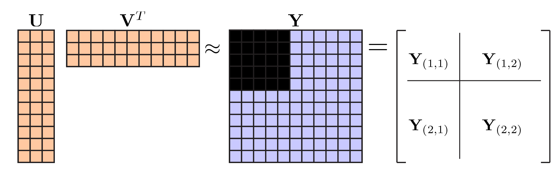Bi-cross-validation holdout pattern. .

This holdout pattern was considered by Owen & Perry (2009) who attribute the basic idea to Gabriel (although he only proposed holding out a single entry of the matrix, rather than a block). A neat thing about this approach is that one can fit a PCA or NMF model to the (fully observed) bottom right block, $\mathbf{Y}_{(2,2)}$, and then use that model to predict the (held-out test) block $\mathbf{Y}_{(1,1)}$ based on the off-diagonal blocks. Understanding how this works takes a bit of effort, but the take-home message is that their approach offers significant speed ups to what I outlined above.

Fu & Perry (2017) recently extended the above idea to K-means clustering. Perry’s PhD thesis is another good reference.

Option 3: imputation

Another viable option is to reformulate the optimization problem to circumvent the problem of missing data. We saw above and in the accompanying post that it is tricky to optimize $\lVert \mathbf{M} \circ \left ( \mathbf{U} \mathbf{V}^T - \mathbf{Y} \right ) \rVert_F^2 $ directly — the Hadamard product complicates things!

We can instead choose to solve the following optimization problem:

where we have added a new variable $\mathbf{Z}$ that is the same shape as $\mathbf{Y}$. Now we can cyclically optimize over $\mathbf{U}$, $\mathbf{V}$, and $\mathbf{Z}$. Each update over $\mathbf{U}$ and $\mathbf{V}$ is now easy — whatever you typically use to fit your model works now!

Updating $\mathbf{Z}$ is also very easy. The observed data points, encoded by nonzero entries in $\mathbf{M}$, are constrained to equal the corresponding entries in $\mathbf{Y}$. But the censored data points can be set to whatever we choose. Clearly, to minimize the loss, the best choice is to set these datapoints to our current model estimate. That is:

Upon updating $\mathbf{Z}$ by this rule we can see that $\left ( \mathbf{U} \mathbf{V}^T - \mathbf{Z} \right )_{ij} = 0$ at all missing datapoints. Thus,

which should convince you that the optimization problems in Equations 3 and 4 are indeed equivalent. The overall procedure is summarized in the figure below.

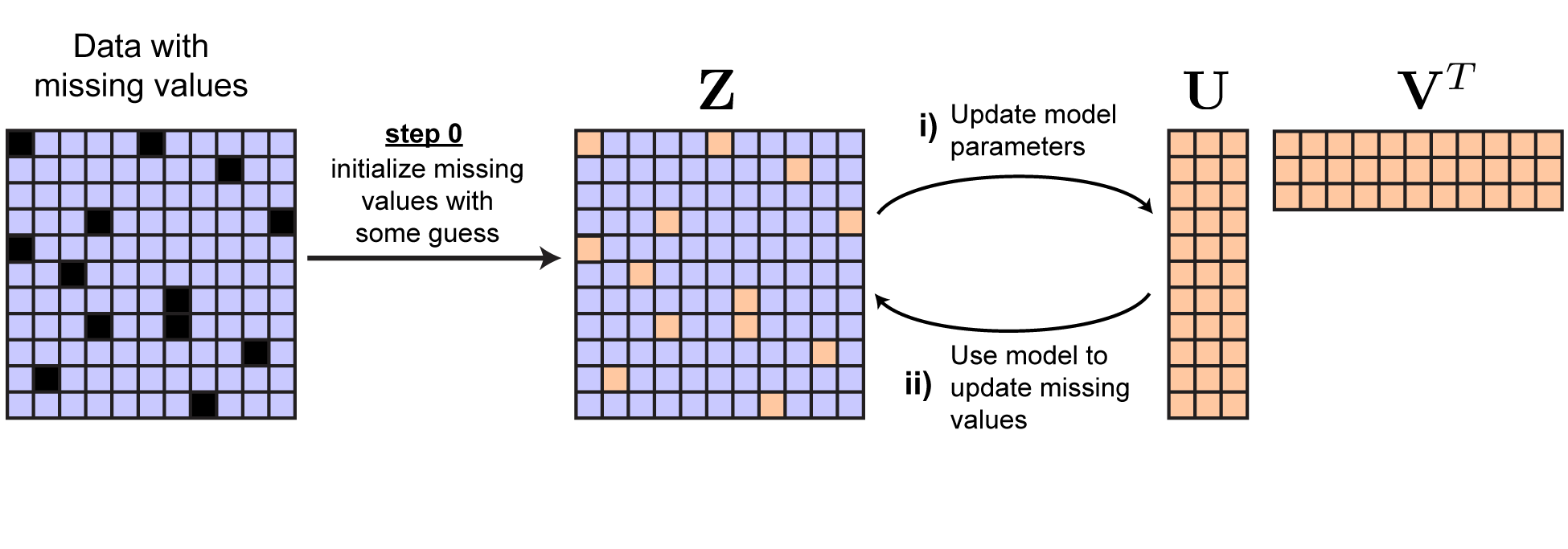Solution by repeated imputation of missing values.

I’ve come to really like this approach for a couple reasons. First, it enables you to re-use the same code for model fitting without masked/missing data entries. Second, it actually can end up being quite fast, since the updates for $\mathbf{U}$ and $\mathbf{V}$ tend to be much faster. For example, doing least squares with missing data involves a nifty, but potentially costly, tensorization step. Similarly, acceleration tricks for NMF optimization (Gillis & Glineur, 2012) don’t nicely extend to the case of missing data. So overall, this approach can offer a good mix of simplicity and efficiency.

Conclusion

Everything here is a brief overview of a topic that has been studied more deeply in the literature. The take-home message is that cross-validation is a bit tricky for unsupervised learning, but there is a simple approach that generalizes to many methods. I just showed you three (PCA, NMF, and $k$-means clustering), but the basic idea applies elsewhere.

Also, there are some very interesting and compelling Bayesian alternatives to this (see Minka, 2000, and the discussion in Murphy’s textbook). I hope to cover those someday in a future post.