Solving Least-Squares Regression with Missing Data

I recently got interested in figuring out how to perform cross-validation on PCA and other matrix factorization models. The way I chose to solve the cross-validation problem (see my other post) revealed another interesting problem: how to fit a linear regression model with missing dependent variables. Since I did not find too many existing resources on this material, I decided to briefly document what I learned in this blog post.

The Problem

We want to solve the following optimization problem, which corresponds to least-squares regression with missing data:

The columns of the matrix $\mathbf{B}$ hold different dependent variables. The columns of the matrix $\mathbf{A}$ hold independent variables. We would like to find the regression coefficients, contained in $\mathbf{X}$, that minimize the squared error between our model prediction $\mathbf{A} \mathbf{X}$ and the dependent variables, $\mathbf{B}$.

However, suppose some entries in the matrix $\mathbf{B}$ are missing. We can encode the missingness with a masking matrix, $\mathbf{M}$. If element $B_{ij}$ is missing, we set $M_{ij} = 0$. Otherwise, we set $M_{ij} = 1$, meaning that element $B_{ij}$ was observed. The “$\circ$” operator denotes the Hadamard product between two matrices. Thus, in equation 1, the masking matrix $\mathbf{M}$ has the effect of zeroing out, or ignoring, the reconstruction error wherever $\mathbf{B}$ has a missing element.

Visually, the problem we are trying to solve looks like this:

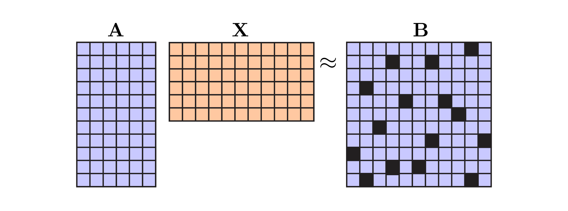Least squares with missing data. Black squares denote missing data values. Note that we only consider missing dependent variables in this post. The masking matrix $\mathbf{M}$ would have zeros along the black squares and ones elsewhere.

Though it is not entirely correct, you can think of the black boxes in the above visualization as NaN entries in the data matrix. The black boxes are not zeros. If we replaced the NaNs with zeros, we obviously get the wrong result. The missing datapoints could be any (nonzero) value!

The optimization problem shown in equation 1 is convex, and it turns out we can derive an analytic solution (similar to least-squares in the abscence of missing data). We can differentiate the objective function with respect to $\mathbf{X}$ and set the gradient to zero. Solving the resulting expression for $\mathbf{X}$ will give us the minimum of the optimization problem. After some computations (see the appendix for details) we arrive at:

which we’d like to solve for $\mathbf{X}$. Computing the right hand side is easy, but the Hadamard product mucks things up on the left hand size. So we need to do some clever rearranging. Consider element $(i,j)$ on the left hand side above, which looks like this:

Pulling the sum over $p$ out front, we get a nicer expression:

The term in square brackets has three indices: $i$, $p$, and $j$. So it is a tensor! In fact, the above expression is the multiplication of a matrix, $\mathbf{X}$, with a tensor. See section 2.5 of Kolda & Bader (2009) for a summary of this matrix-tensor operation.

Let’s define the tensor as $\mathcal{T}$:

I suggestively decided to index along mode $j$ in the superscript. Consider a slice through the tensor at index $j$. We are left with a matrix, which can be written as:

Where $\text{diag}(\cdot)$ transforms a vector into a diagonal matrix (a standard operation available in MATLAB/Python). Let’s draw an illustration to summarize what we’ve done so far:

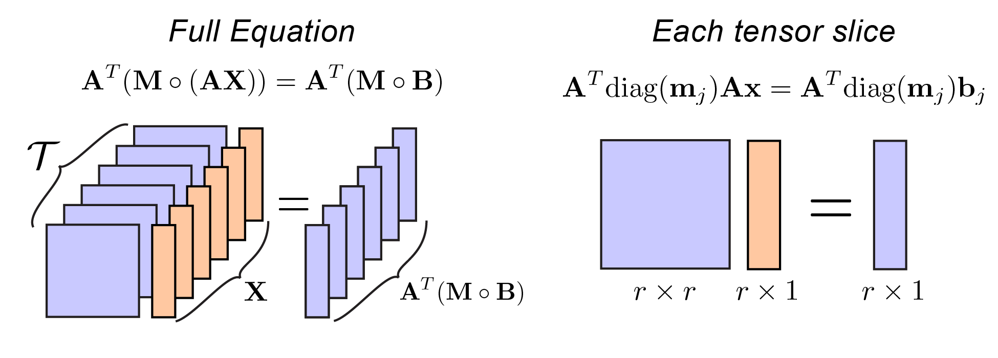Representation of equation 2 using the tensor described in equation 3.

It turns out that we are basically done due to the magic of numpy broadcasting. We simply need to construct the tensor, $\mathcal{T}$, and the matrix $\mathbf{A}^T (\mathbf{M} \circ \mathbf{B})$, and then call numpy.linalg.solve. The following code snippet does exactly this:

def censored_lstsq(A, B, M):
    """Solves least squares problem subject to missing data.

    Note: uses a broadcasted solve for speed.

    Args
    ----
    A (ndarray) : m x r matrix
    B (ndarray) : m x n matrix
    M (ndarray) : m x n binary matrix (zeros indicate missing values)

    Returns
    -------
    X (ndarray) : r x n matrix that minimizes norm(M*(AX - B))
    """

    # Note: we should check A is full rank but we won't bother...

    # if B is a vector, simply drop out corresponding rows in A
    if B.ndim == 1 or B.shape[1] == 1:
        return np.linalg.leastsq(A[M], B[M])[0]

    # else solve via tensor representation
    rhs = np.dot(A.T, M * B).T[:,:,None] # n x r x 1 tensor
    T = np.matmul(A.T[None,:,:], M.T[:,:,None] * A[None,:,:]) # n x r x r tensor
    return np.squeeze(np.linalg.solve(T, rhs)).T # transpose to get r x n

Since $\mathbf{A}^T \text{diag}(\mathbf{m}_{j}) \mathbf{A}$ is symmetric and positive definite we could use the Cholesky decomposition to solve the system rather than the more generic numpy solver. If anyone has an idea/comment about how to implement this efficiently in Python, I’d love to know!

Here’s my rough analysis of time complexity (let me know if you spot an error):

• The Hadamard product M * B is $\mathcal{O}(mn)$
• Strassen fanciness aside, matrix multiplication np.dot(A.T, M * B) is $\mathcal{O}(mnr)$
• The broadcasted Hadamard M.T[:,:,None] * A[None,:,:] is $\mathcal{O}(mnr)$
• Building the tensor involves n matrix multiplications, totalling $\mathcal{O}(m n r^2)$.
• Then solving each of the n slices in the tensor takes $\mathcal{O}(n r^3)$.

So the total number of operations is $\mathcal{O}(n r^3 + m n r^2)$. In practice, this does run noticeably slower than a regular least-squares solve, so I’d love suggestions for improvements!

A less fun solution

There is another simple solution to this least-squares problem, but it doesn’t involve tensors and requires a for loop. The idea is to solve for each column of $\mathbf{X}$ sequentially. Let $\mathbf{x}_i$ be the $i^\text{th}$ column of $\mathbf{X}$ and let $\mathbf{b}_i$ likewise by the $i^\text{th}$ column of $\mathbf{B}$. It is intuitive that the least-squares solution for $\mathbf{x}_i$ is given by dropping the rows of $\mathbf{A}$ where $\mathbf{b}_i$ has a missing entry.

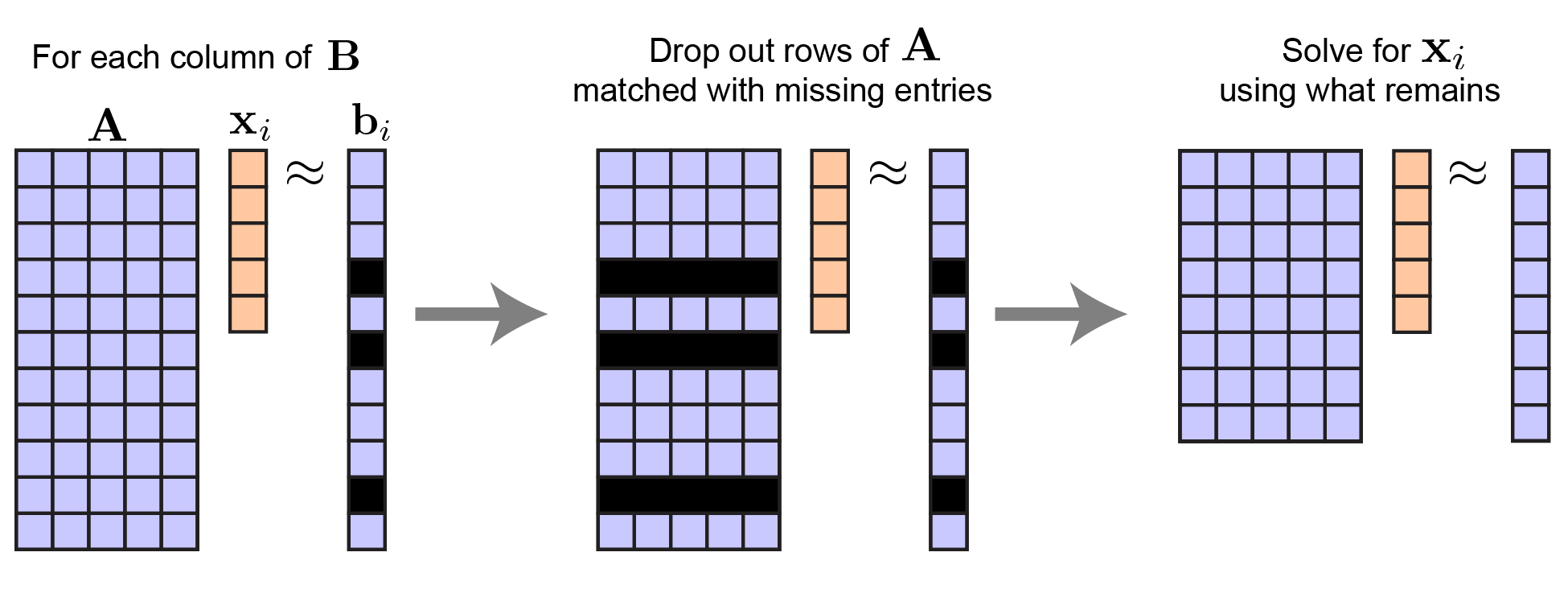Least squares with missing data for a single column of $B$.

def censored_lstsq_slow(A, B, M):
    """Solves least squares problem subject to missing data.

    Note: uses a for loop over the columns of B, leading to a
    slower but more numerically stable algorithm

    Args
    ----
    A (ndarray) : m x r matrix
    B (ndarray) : m x n matrix
    M (ndarray) : m x n binary matrix (zeros indicate missing values)

    Returns
    -------
    X (ndarray) : r x n matrix that minimizes norm(M*(AX - B))
    """

    X = np.empty((A.shape[1], B.shape[1]))
    for i in range(B.shape[1]):
        m = M[:,i] # drop rows where mask is zero
        X[:,i] = np.linalg.lstsq(A[m], B[m,i])[0]
    return X

It has a similar complexity of $\mathcal{O}(m n r^2)$, due to solving n least squares equations each with $\mathcal{O}(m r^2)$ operations. Since we have added a for loop this solution does run noticeably slower on my laptop than the first solution for large n. In C++ or Julia, this for loop would be less of a worry.

Also, I think this second (less fun) solution should be more accurate numerically because it does not compute the Gramian, $\mathbf{A}^T \mathbf{A}$, whereas the first method I offered essentially does this. The condition number of the Gramian is the square of the original matrix, $\kappa ( \mathbf{A}^T \mathbf{A}) = \kappa (\mathbf{A})^2$, so the result will be less stable. This is why some least-squares solvers do not use the normal equations under the hood (they instead use QR decomposition).

Conclusion

I’ve outlined a couple of simple ways to solve the least-squares regression problem with missing data in the dependent variables. The two Python functions I offered have a tradeoff in speed and accuracy, and while the code could certainly be further optimized - I expect these functions will work well enough for some simple applications.

Appendix

This appendix contains some simple manipulations on the objective function:

Let’s define $\mathbf{E} = \mathbf{A} \mathbf{X} - \mathbf{B}$, which is a matrix of unmasked residuals. Then, since $m_{ij} \in \{0, 1\}$ the objective function simplifies:

We are using $\textbf{Tr} [ \cdot ]$ to denote the trace of a matrix, and the fact that $\lVert \mathbf{X} \lVert^2_F = \textbf{Tr} [\mathbf{X}^T \mathbf{X}]$ for any matrix $\mathbf{X}$. Now we’ll substitute $\mathbf{A}\mathbf{X} - \mathbf{B}$ back in and expand the expression:

Now we differentiate these three terms with respect to $\mathbf{X}$. The term on the right goes to zero as it does not depend on $\mathbf{X}$. The term in the middle is quite standard and can be found in the matrix cookbook:

The first term in equation 5 is a bit of a pain and we’ll derive it manually. We resort to a summation notation and compute the partial derivative with respect to element $(a, b)$ of $\mathbf{X}$:

Now we’ll pull all of the sums out front and make our notation more compact. Then we’ll differentiate:

By inspection, you can convince yourself that this final expression maps onto $2 \mathbf{A^T (\mathbf{M} \circ (\mathbf{A} \mathbf{X}))}$ in matrix notation. Combining this result with equation 6, we arrive at:

Which immediately implies equation 2 in the main text.