A Short Introduction to Optimal Transport and Wasserstein Distance

These notes provide a brief introduction to optimal transport theory, prioritizing intuition over mathematical rigor. A more rigorous presentation would require some additional background in measure theory. Other good introductory resources for optimal transport theory include:

• Peyré & Cuturi (2019), “Computational Optimal Transport”, Foundations and Trends® in Machine Learning: Vol. 11: No. 5-6, pp 355-607.
• Some introductory lectures.
  • Marco Cuturi. MLSS Africa 2019.   Video Part I – Video Part II
  • Marco Cuturi. MLSS Tübingen 2020.   Video Part I – Video Part II
  • Gabriel Peyré. Talk at the Alan Turing Institute.   Video

Why Optimal Transport Theory?

A fundamental problem in statistics and machine learning is to come up with useful measures of “distance” between pairs of probability distributions. Two desirable properties of a distance function are symmetry and the triangle inequality. Unfortunately, many notions of “distance” between probability distributions do not satisfy these properties. These weaker notions of distance are often called divergences. Perhaps the most well-known divergence is the Kullback-Lieibler (KL) divergence:

Where $P$ and $Q$ here denote probability distributions. While the KL divergence is incredibly useful and fundamental in information theory, it also has its shortcomings.

For instance, one of the first things we learn about the KL divergence is that it is not symmetric, \(D_{KL}(P \| Q) \neq D_{KL}(Q \| P)\). This is arguably not a huge problem, since various symmetrized analogues to the KL divergence exist. A bigger problem is that the divergence may be infinite if the support of $P$ and $Q$ are not equal. Below we sketch three examples of 1D distributions for which \(D_{KL}(P \| Q) = D_{KL}(Q \| P) = +\infty\).

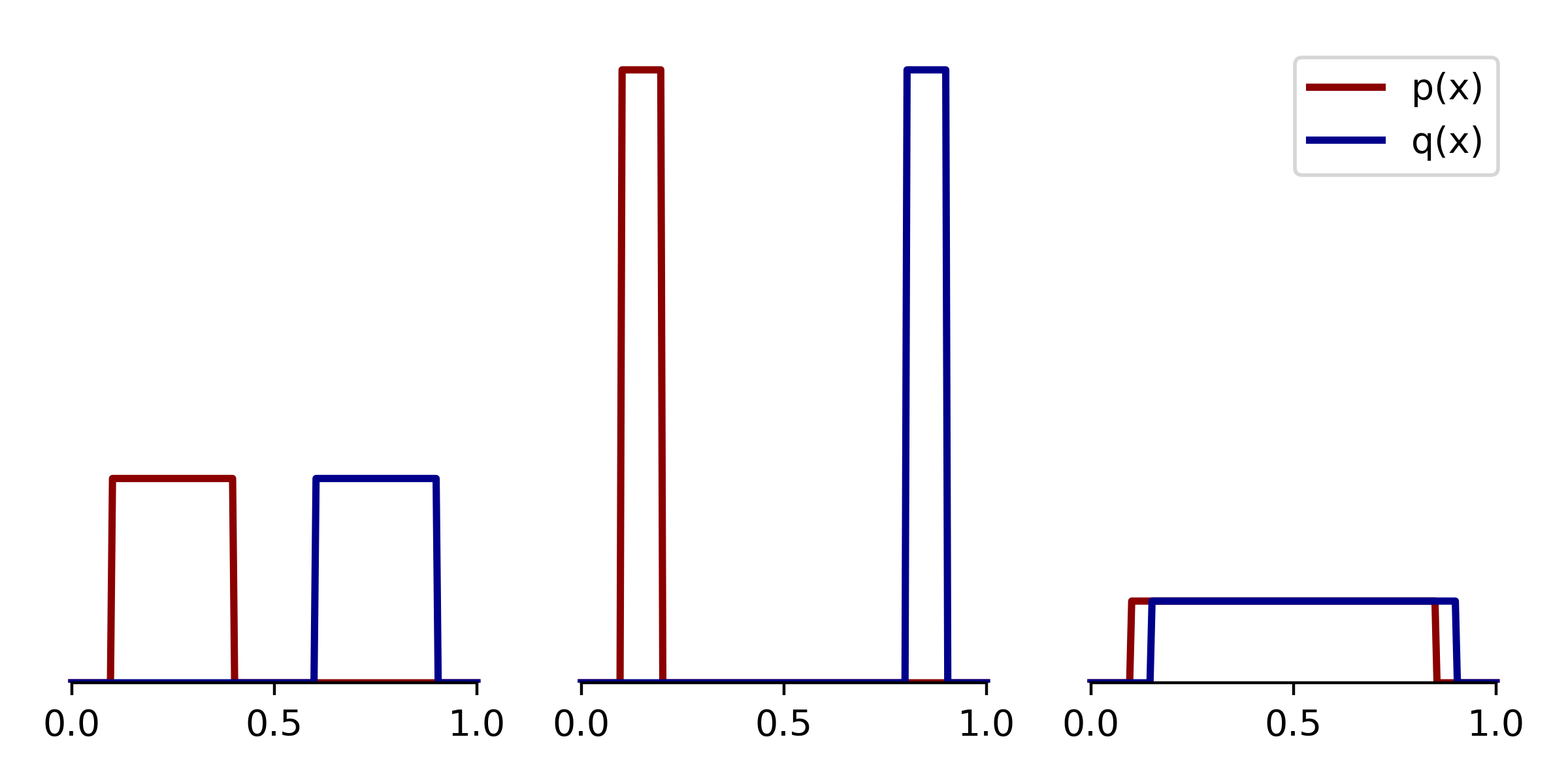Three examples with infinite KL divergence. These density functions are infinitely far apart according to KL divergence, since in each case there exist intervals of $x$ where $q(x) = 0$ but $p(x)>0$, leading to division by zero.

Intuitively, some of these distribution pairs seem “closer” to each other than others. But the KL divergence says that they are all infinitely far apart. One way of circumventing this is to smooth (i.e. add blur to) the distributions before computing the KL divergence, so that the support of $P$ and $Q$ matches. However, choosing the bandwidth parameter of the smoothing kernel is not always straightforward.

Optimal transport theory is one way to construct an alternative notion of distance between probability distributions. In particular, we will encounter the Wasserstein distance, which is also known as “Earth Mover’s Distance” for reasons which will become apparent. This distance is not only symmetric, but also satisfies the triangle inequality.

Interest in optimal transport seems to have rapidly increased in recent years, with applications arising in imaging (Lee et al., 2020), generative models (Arjovsky et al., 2017), and biological data analysis (Schiebinger, 2019), to name a few.

An example transport problem in 2D

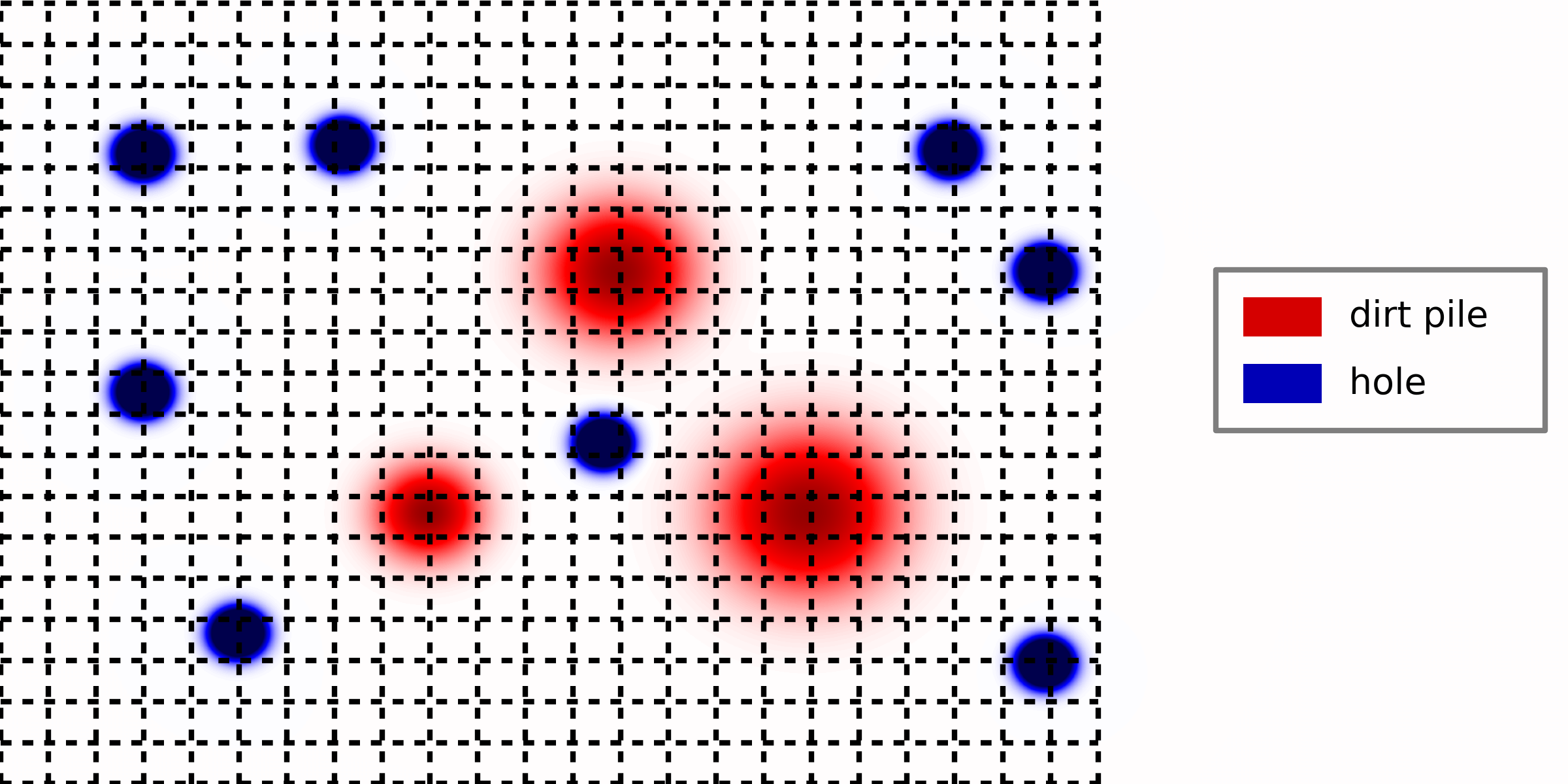
One of the nice aspects of optimal transport theory is that it can be grounded in physical intuition through the following thought experiment. Suppose we are given the task of filling several holes in the ground. The image below shows an overhead 2D view of this scenario — the three red regions correspond to dirt piles, and the eight blue regions correspond to holes.

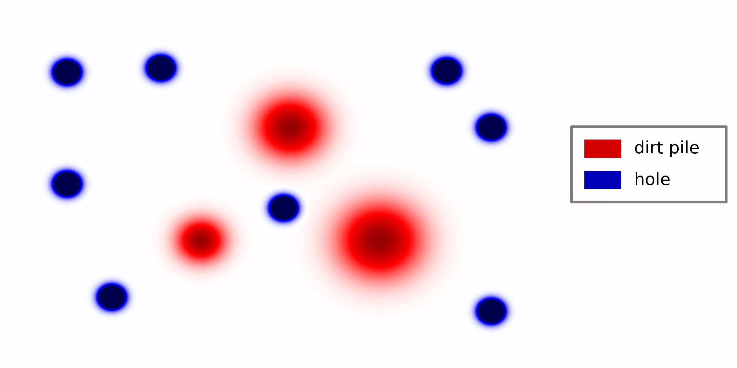Toy example in 2D. Overhead view of piled dirt (red) which must be transported to fill holes (blue).

Our goal is to come up with the most efficient transportation plan to which moves the dirt to fill all the holes. We assume the total volume of the holes is equal to the total volume of the dirt piles. In case it isn’t clear where this is going — you should think of the piles as the probability density function of $P$ and the holes as the probability density function of $Q$.^[1]

The “most efficient” plan is the one that minimizes the total transportation cost. To quantify this, let’s say the transportation cost $C$ of moving 1 unit of dirt from $(x_0, y_0) \rightarrow (x_1, y_1)$ is given by the squared Euclidean distance:

Other choices for the cost function are possible, but we will stick with this simple case. Now we’ll define the transportation plan $T$, which tells us how many units of dirt to move from $(x_0, y_0) \rightarrow (x_1, y_1)$. For example, if the plan specifies:

then we intend to move $w$ units of dirt from position $(x_0, y_0) \rightarrow (x_1, y_1)$. For this to be a valid plan, we must start with at least $w$ units of dirt at $(x_0, y_0)$, and the depth of the hole at $(x_1, y_1)$ must correspond to at least $w$ units. Also, we are only allowed to move positive units of dirt. We do allow dirt originating from $(x_0, y_0)$ to be split among multiple destinations.^[2] In our 2D overhead view, we can visualize the transport $(x_0, y_0) \rightarrow (x_1, y_1)$ with an arrow like so:

Example transport path. The arrow schematizes $w$ units of dirt being transported from location (x0, y0) to (x1, y1). A complete transport plan specifies transport paths like this over all pairs of locations.

The transportation plan, $T$, specifies an arrow like this from every possible starting position to every possible destination. Further, in addition to being nonnegative $T(x_0, y_0, x_1, y_1) \geq 0$, the plan must satisfy the following two conditions:

Where $p(\cdot, \cdot)$ and $q(\cdot, \cdot)$ are density functions encoding the units of dirt and hole depth at each 2D location. Intuitively, the first constraint says that the amount of piled dirt at \((x_0, y_0)\) is “used up” or transported somewhere. The second constraint says that the hole at \((x_1, y_1)\) is “filled up” with the required amount of dirt (no more and no less).

Suppose we are given a function $T$ that satisfies all of these conditions (i.e. we are given a feasible transport plan).^[3] Then the overall transport cost is given by:

This expression should be intuitive. In essence, it states that that for every pointwise transportation \((x_0, y_0) \rightarrow (x_1, y_1)\) we multiply the amount of dirt transported, given by $T$, by the per unit transport cost, given by $C$. Integrating over all possible origins and destinations gives us the total cost.

We’ve now fully formulated the optimal transport problem in 2D. Taking a step back, here are a few notes of interest about the problem:

• At first glance, finding the optimal transport plan $T$ might appear to be a really hard problem! However, we will show in the next section that, after discretizing the problem, finding the best transport plan amounts to solving a linear program. Perhaps easier than you might have first guessed!

• We can interpret the transport plan as a probability distribution. Specifically, if $P$ and $Q$ are probability distributions over some space $\mathcal{X}$, then the transport plan can be viewed as a probability distribution over $\mathcal{X} \times \mathcal{X}$ where the operator “$\times$” denotes the Cartesian product (see also product measurable space). In our example above the space $\mathcal{X}$ corresponds to 2D Euclidean space, $\mathbb{R}^2$, and thus the transport plan a probability distribution on $\mathbb{R}^2 \times \mathbb{R}^2$ (which is isomorphic to 4D space, $\mathbb{R}^4$).

• The total transportation cost overcomes the two weaknesses of KL divergence we discussed at the beginning of this post. First, since the cost function $C$ is symmetric, the overall cost to transport $P \rightarrow Q$ is the same as transporting $Q \rightarrow P$. We will revisit this point again, but for now we schematize a simple 1D example to hopefully provide sufficient intuition for the symmetry:

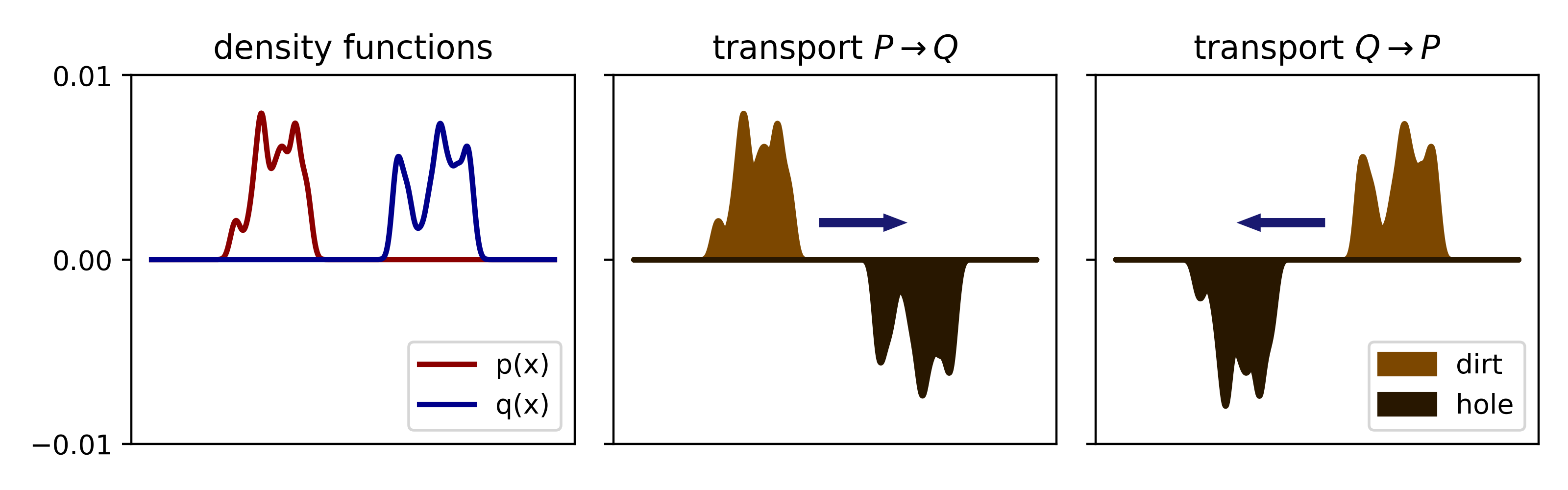Transport costs are symmetric. The density functions associated with $P$ and $Q$ are plotted on the left. In the middle and on the right we schematize the two possible transport problems. The symmetries in the problem (e.g. it is equally costly to move dirt left vs. right) mean that these two problems result in equivalent optimal transport costs.

• Recall the second shortcoming of KL divergence — it was infinite for a variety of distributions with unequal support. Below we revisit the three simple 1D examples we showed at the beginning and compute the Wasserstein distance between them. Not only is the Wasserstein distance finite in all cases, but the distances agree with our natural intuitions: the panel on the right results in the smallest Wasserstein distance, while the middle panel shows the largest distance.

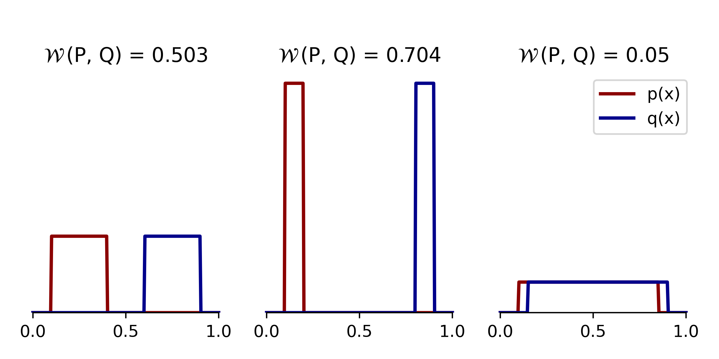Examples in 1D revisited Unlike KL divergence, the Wasserstein distances in these examples are finite and intuitive.

Optimal transport between discrete distributions

In general, identifying optimal transport plans between continuous distributions is challenging, and is only analytically tractable in a few special cases.^[4] However, we can often compute reasonable estimates of the optimal transport cost by discretizing the problem. For our 2D example above, we could use a 2D grid for this discretization:

In essence, at the price of introducing some discretization error, we have reduced the problem to transporting a dirt among a finite number of spatial bins. Assuming there are a total of $n$ bins, with positions \(\{\mathbf{x}_i\}_{i=1}^n\), then the discretized distributions of interest are:

where \(\delta_\mathbf{x}\) denotes a Dirac delta function placed at a location $\mathbf{x} \in \mathbb{R}^2$. In other words, we place delta functions at the center of each spatial bin and weight them by the probability mass assigned to that bin.

So we’ve reduced the problem to discrete transport over $n$ spatial bins. Now, we can enumerate all \((n^2 - n) / 2\) pairs of spatial bins and compute their transportation costs. The cost from moving one unit of dirt from bin $i$ to bin $j$ (or vice versa) is:

This symmetric cost matrix is directly analogous to the cost function we used in the previous section, and hence we re-use the letter $C$ without introducing any confusion. Likewise, the transport plan in the discrete case reduces to a matrix, $\mathbf{T} \in \mathbb{R}^{n \times n}$. The total cost of a transport plan is then:

where we have used the usual Frobenius inner product between two matrices. The optimal transport plan is therefore given by the following optimization problem:

As before, the constraints ensure that the marginal distributions of the transport plan match $P$ and $Q$. These constraints are analogous to equations 4 & 5 from the previous section — at each location the transport plan must distribute the exact amount of initial dirt and must match the final amount of desired dirt. We can state the optimization problem even more compactly if we let $\boldsymbol{1}$ denote a vector of ones:

Letting \(\mathbf{T}^*\) denote the solution to the above optimization problem, the Wasserstein distance is defined as:^[5]

It is easy to see that $\mathcal{W}(P, Q) = 0$ if $P = Q$, since in this case we would have \(\mathbf{T}^* = \text{diag}(\mathbf{p}) = \text{diag}(\mathbf{q})\) and the diagonal entries of $\mathbf{C}$ are zero. It is also easy to see that $\mathcal{W}(P, Q) = \mathcal{W}(Q, P)$ for any choice of $P$ and $Q$ since the optimal transport plans are simply transposes of each other and $\mathbf{C}$ is a symmetric matrix. Proving the triangle inequality is slightly more involved and beyond the scope of these notes.

Solving the Optimization Problem

The optimization problem presented above is a linear program, so it can be solved in polynomial time by general-purpose algorithms. Here we’ll use scipy.optimize.linprog(...) for demonstration purposes, but readers should note that there are more efficient and specialized algorithms (e.g., Orlin’s algorithm; see also chapter 3 of Peyré & Cuturi). The function below computes the Wasserstein distance between two discrete distributions with probability mass functions p and q and with atoms located at x.

def demo_wasserstein(x, p, q):
    """
    Computes order-2 Wasserstein distance between two
    discrete distributions.

    Parameters
    ----------
    x : ndarray, has shape (num_bins, dimension)
    
        Locations of discrete atoms (or "spatial bins")

    p : ndarray, has shape (num_bins,)

        Probability mass of the first distribution on each atom.

    q : ndarray, has shape (num_bins,)

        Probability mass of the second distribution on each atom.

    Returns
    -------
    dist : float

        The Wasserstein distance between the two distributions.

    T : ndarray, has shape (num_bins, num_bins)

        Optimal transport plan. Satisfies p == T.sum(axis=0)
        and q == T.sum(axis=1).

    Note
    ----
    This function is meant for demo purposes only and is not
    optimized for speed. It should still work reasonably well
    for moderately sized problems.
    """

    # Check inputs.
    if (abs(p.sum() - 1) > 1e-9) or (abs(p.sum() - q.sum()) > 1e-9):
        raise ValueError("Expected normalized probability masses.")

    if np.any(p < 0) or np.any(q < 0):
        raise ValueError("Expected nonnegative mass vectors.")

    if (x.shape[0] != p.size) or (p.size != q.size):
        raise ValueError("Dimension mismatch.")

    # Compute pairwise costs between all xs.
    n, d = x.shape
    C = squareform(pdist(x, metric="sqeuclidean"))

    # Scipy's linear programming solver will accept the problem in
    # the following form:
    # 
    # minimize     c @ t        over t
    # subject to   A @ t == b
    #
    # where we specify the vectors c, b and the matrix A as parameters.

    # Construct matrices Ap and Aq encoding marginal constraints.
    # We want (Ap @ t == p) and (Aq @ t == q).
    Ap, Aq = [], []
    z = np.zeros((n, n))
    z[:, 0] = 1

    for i in range(n):
        Ap.append(z.ravel())
        Aq.append(z.transpose().ravel())
        z = np.roll(z, 1, axis=1)

    # We can leave off the final constraint, as it is redundant.
    # See Remark 3.1 in Peyre & Cuturi (2019).
    A = np.row_stack((Ap, Aq))[:-1]
    b = np.concatenate((p, q))[:-1]

    # Solve linear program, recover optimal vector t.
    result = linprog(C.ravel(), A_eq=A, b_eq=b)

    # Reshape optimal vector into (n x n) transport plan matrix T.
    T = result.x.reshape((n, n))

    # Return Wasserstein distance and transport plan.
    return np.sqrt(np.sum(T * C)), T

An Example in 1D

To demonstrate what this looks like, let’s first consider a 1D example. On the left panel below we show two probability mass functions defined on the interval $[0, 1]$. On the right, visualize the cost matrix $\mathbf{C}$ along with the same density functions (one up top and other flipped vertically). The cost is zero along the diagonal of $\mathbf{C}$ since it costs us nothing to move mass zero units of distance. Since we define the transportation cost as squared Euclidean distance, moving vertically or horizontally off the diagonal increases the cost quadratically.

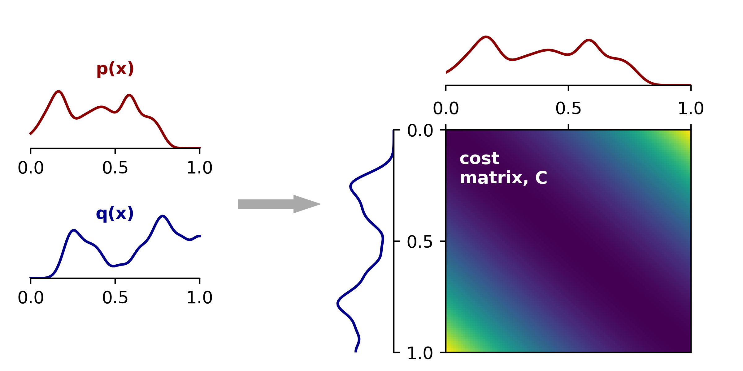Transport cost matrix in 1D Left, density functions for two distributions $P$ and $Q$ defined on the unit interval. Right, cost matrix showing squared Euclidean distances between all pairs of points.

The figure above displays all the necessary ingredients for us to find the optimal transport plan: two target marginal distributions $\mathbf{p}$ and $\mathbf{q}$ and the cost matrix $\mathbf{C}$. We input these three ingredients into our the linear programming solver and are given back the optimal transport plan \(\mathbf{T}^*\). This transport plan is a matrix the same size as $\mathbf{C}$ and is shown below on the right:

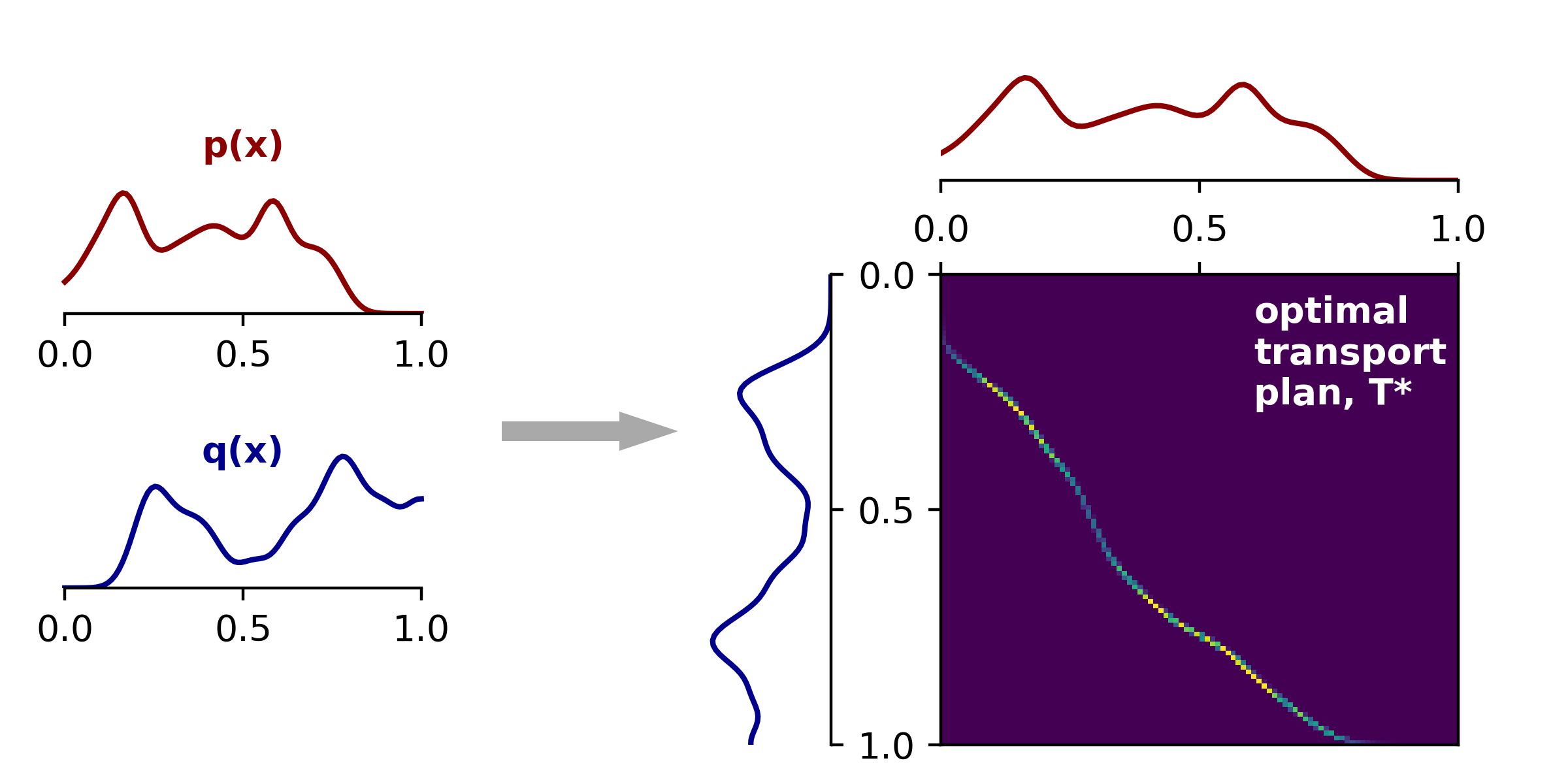Optimal transport plan matrix in 1D Left, same density functions as above. Right, transport plan matrix, $\mathbf{T}^*$. Entry $(i,j)$ in this matrix specifies how much mass in bin $i$ of $Q$ should be transported to bin $j$ of $P$. (Or vice versa, due to the symmetry we've discussed.)

By inspecting this transport plan, we can appreciate a few high-level patterns. First, \(\mathbf{T}^*\) is very sparse, and nonzero entries trace out a curved path from the upper left to the lower right corner. This is intuitive — the masses at two nearby locations have a similar transport cost no matter what we choose to be the destination. Thus, we would expect their optimal destinations to be close together (especially because the marginal densities are smooth in this example).

Second, the largest peaks in \(\mathbf{T}^*\) (the parts colored yellow) correspond to peaks in the marginal densities. Conversely, dark spots in the transport plan correspond to troughs in $\mathbf{p}$ and $\mathbf{q}$. This is also intuitive because the transport plan is constrained to match these marginal distributions; expressed in Python, we have T.sum(axis=0) == p and T.sum(axis=1) == q (up to floating point precision). Finally, the nonzero elements in \(\mathbf{T}^*\) lie below the diagonal. This is because most of the mass in $\mathbf{p}$ is to the left of the mass in $\mathbf{q}$.

An Example in 2D

Now let’s return to our original 2D problem and see what the solution looks like in this more complex setting. As mentioned before, we will discretize our problem into spatial bins. Here, I’ve chosen a 20 x 20 grid, which is rather coarse-grained, but it works for demonstration purposes. The left panels shows the discretized 2D heat maps — $\mathbf{p}$ corresponds to the three dirt piles, and $\mathbf{q}$ corresponds to the scattered holes. On the right, we plot these same densities after flattening these 2D densities into 1D vectors, and also plot the cost matrix, $\mathbf{C}$. Since we have a 20 x 20 discrete grid, there are a total of 400 bins, and thus $\mathbf{C}$ is a 400 x 400 matrix.

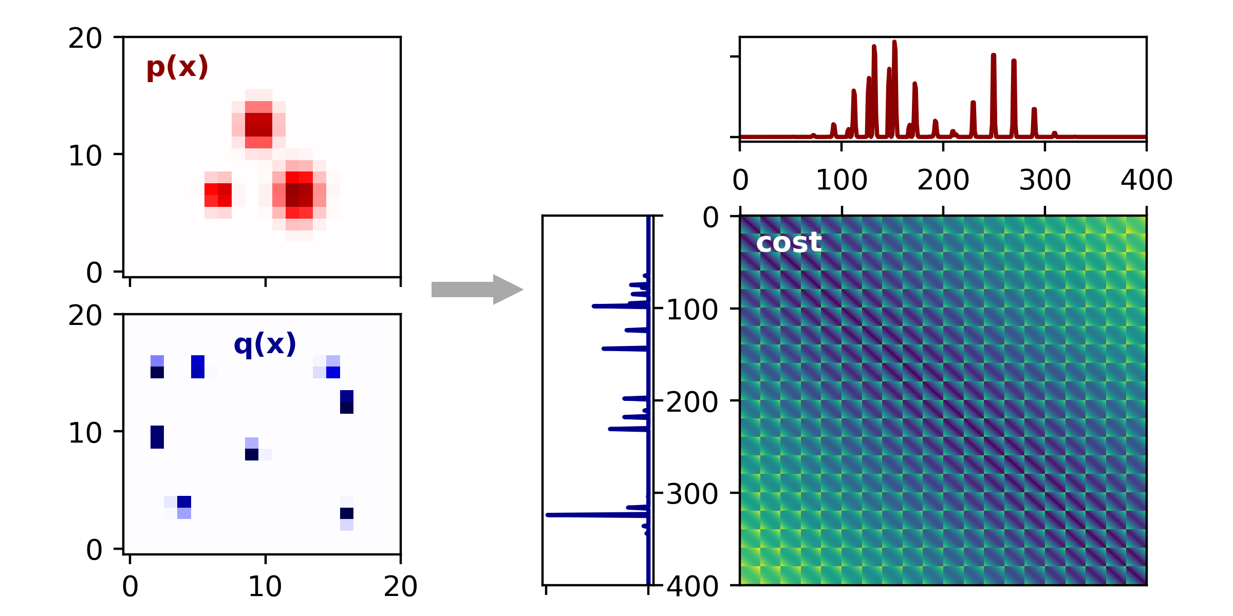Transport cost matrix in 2D Left, Density functions for $P$ and $Q$. These are discretized verions of our original problem. Right, symmetric matrix of transport costs. The blocky structure arises because we had to flatten the 2D grid of bins defining $P$ and $Q$.

Because these visualizations reduce the 2D distributions down to a single dimension, they are a bit more complicated and tricky to interpret than the 1D case. Here I linearized the 2D grid of bins by the standard numpy.ravel(), so after a bit of reflection the blocky structure of the cost matrix above should make since. Rather than getting lost in these details, the important point is that we have reduced the 2D problem to something similar to the 1D example we considered in the last section, and we can use the same code to identify the optimal transport plan, \(\mathbf{T}^*\). Doing this, we obtain the following:

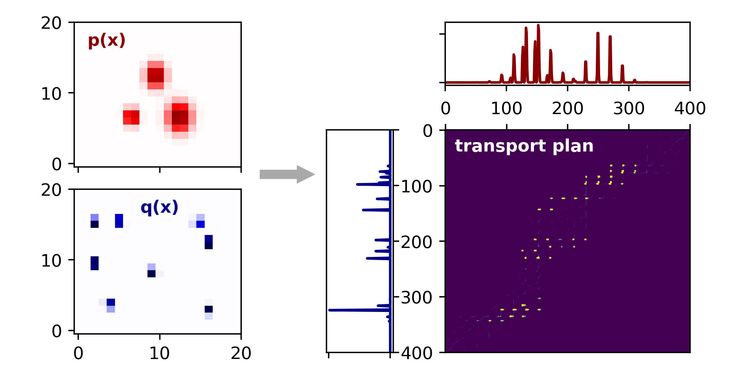Optimal transport plan in 2D Left, same 2D density functions as above. Right, transport plan matrix, $\mathbf{T}^*$ found by linear programming.

It is pretty difficult to visually interpret this optimal transport plan as it is extremely sparse — in fact, I had to add a little bit of Gaussian blur to the heatmap so that the yellow spots, corresponding to peaks in \(\mathbf{T}^*\), are visible. Regardless, it is very satisfying that the same linear programming approach worked for us as in the 1D example above. If we wanted to, we could now take the inner product between \(\mathbf{T}^*\) and $\mathbf{C}$ and then take the square root to arrive at the Wasserstein distance between $P$ and $Q$.

Though this is enough to demonstrate the basic idea, it would be a bit dissatisfying to end without something a little more intuitive. Below, I took the largest 80 entries of the optimal transport plan, which is plotted above as a heatmap. Each of these entries, \(\mathbf{T}^*_{ij}\), specifies an origin (bin $i$) and a destination (bin $j$). When we overlay these 80 arrows on top of our (discretized) 2D densities, we get very intuitive and satisfying result:

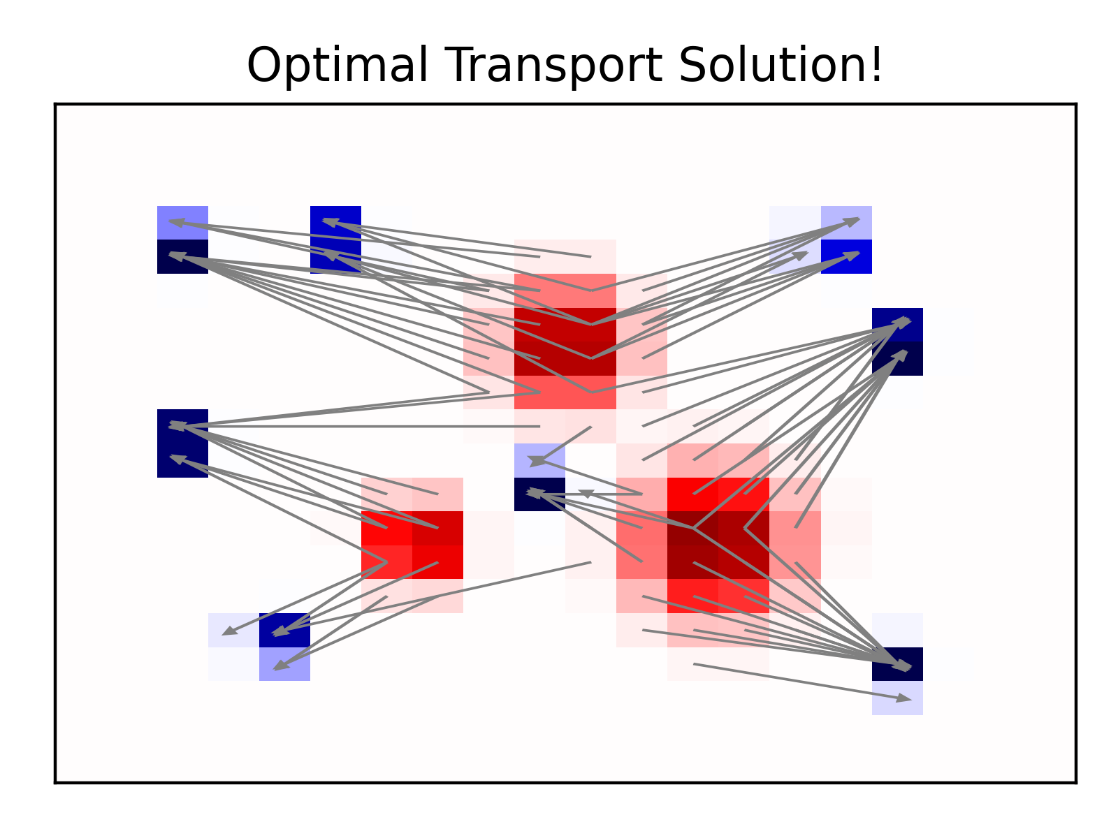A simpler visualization of the optimal transport plan for the (discretized) 2D toy problem.

Entropy Regularization

Before concluding, I want to quickly mention an important innovation that has galvanized recent work on optimal transport in machine learning. Very briefly, the idea is to penalize transport plans with small Shannon entropy. To do this we modify the optimization problem as follows:

Here, $\epsilon > 0$ is the strength of the regularization penalty and \(H(\mathbf{T}) = -\sum_{ij} \mathbf{T}_{ij} \log \mathbf{T}_{ij}\) is the Shannon entropy.^[6] As $\epsilon \rightarrow 0$, we of course cover our original optimal transport problem. As $\epsilon \rightarrow \infty$ it can be shown that the optimal transport plan is given by \(\mathbf{T}_{ij}^* = \mathbf{p}_i \mathbf{q}_j\), so intuitively the problem becomes progressively easier to solve as we increase $\epsilon$. You can think of the regularization term as reducing sparsity in optimal transport plan and discouraging the solution from hiding out in the sharp edges of the polytope defined by the linear constraints of the problem.

The figure below shows the effect of decreasing the regularization strength for a simple 1D optimal transport problem. The marginal densities are shown by the blue and red lines on the bottom panels. The colored heatmaps (top) and 2d surface plots (bottom) visualize the optimal transport plan for various values of $\epsilon$.

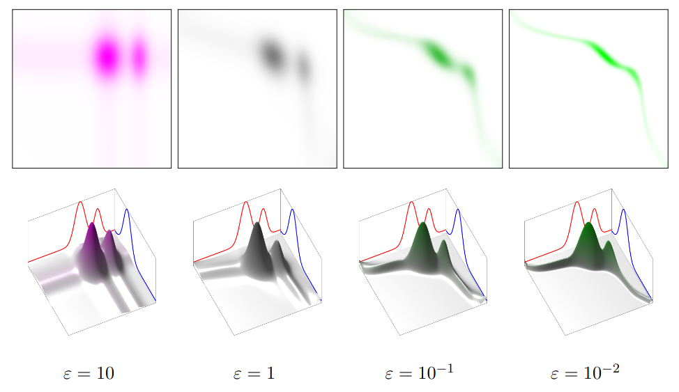Effect of entropic regularization on transport (reproduced from Peyré & Cuturi, Fig. 4.2)

The computational advantages of entropy regularization are substantial for high-dimensional data. If we discretize the space into $d$ bins (as we did in the previous section) then we can expect the computational expense to be $O(d^3 \log d)$.^[7] In contrast, we can expect nearly linear time convergence after adding the entropy regularization, as established by recent work (Altschuler et al., 2019 ; Dvurechensky et al., 2019). Chapter 4 of Peyré & Cuturi (2019) provides a good introduction for the algorithmic tricks and interpretations of this entropy-regularized problem.

Footnotes

[1] Or vice versa! It shouldn’t be hard to see that the problem is entirely symmetric — it would cost us the same to transport the dirt back out of the holes as it did to transport the dirt there in the first place, so we can think about transport in either direction as being equivalent.

[2] Allowing dirt to be split in this fashion corresponds to the Kanotorovich formulation of the transport problem, which is distinct from the original formulation which given by Gaspard Monge. We stick to Kanotorovich’s formulation because it is more analytically and computationally tractable (and thus more common in modern applications).

[3] One might wonder — does a feasible transport plan always exist? Yes! One can check that the product measure, \(T(x_0, y_0, x, y) = p(x_0, y_0) q(x_1, y_1)\), satisfies all the required constraints.

[4] There are two notable cases where optimal transport plans can be computed analytically. We state these cases briefly here; further details and references can be found in (Peyré & Cuturi, 2019; Remarks 2.30 and 2.31).

Univariate distributions. Let $f^{-1}(\cdot)$ and $g^{-1}(\cdot)$ denote the inverse c.d.f.s of two univariate distributions. Then, the order-$p$ Wasserstein distance between the distributions is given by $(\int_0^1 |f^{-1}(y) - g^{-1}(y)|^p dy )^{1/p}$.
Gausssian Distributions. Given two normal distributions with means $(\mu_1, \mu_2)$ and covariances $(\Sigma_1, \Sigma_2)$, then the (second order) Wasserstein distance between the distributions is: \((\Vert \mu_1 - \mu_2 \Vert_2^2 + \mathcal{B}(\Sigma_1, \Sigma_2)^2)^{1/2}\) where $\mathcal{B}$ denotes the Bures metric on positive-definite matrices. For univariate normal distributions this simplifies to: \(((\mu_1 - \mu_2)^2 + (\sigma_1 - \sigma_2)^2)^{1/2}\) where $\sigma_1$ and $\sigma_2$ denote the standard deviations. That is, the Wasserstein distance between two 1D gaussians is equal to the Euclidean distance of the parameters plotted in the 2D plane, with axes corresponding to the mean and standard deviation.

[5] Here, we’ve defined the Wasserstein distance for two discrete distributions, but it can also be defined (though not easily computed) for continuous distributions (e.g., see the definition given on Wikipedia). Further, this post only covers the “2nd order” Wasserstein distance for simplicity. More generally, if we define the per-unit costs as \(\mathbf{C}_{ij} = \Vert \mathbf{x}_i - \mathbf{x}_j \Vert^p_2\) then the Wasserstein distance of order $p$ is given by \(\langle \mathbf{T}^*, \mathbf{C} \rangle^{1/p}\). Order $p=1$ Wasserstein distance is also of practical interest since it tends to be more robust to outliers. See chapter 6 of Peyré & Cuturi (2019) for further discussion.

[6] Note that Peyré & Cuturi (2019) define the entropy term slightly differently as \(H(\mathbf{T}) = -\sum_{ij} \mathbf{T}_{ij} \log \mathbf{T}_{ij} + \sum_{ij} \mathbf{T}_{ij}\), but the constraints of our problem imply that \(\sum_{ij} \mathbf{T}_{ij} = 1\) so the only difference is an additive constant. These discrepancies do become important in other cases, such as in the case of unbalanced optimal transport (see section 10.2 of Peyré & Cuturi, 2019).

[7] This is the computational complexity of Orlin’s algorithm which appears to be the current state-of-the-art based on the discussion in Altschuler et al. 2019.